Computing The Laplacian
This post is going to be somewhat longer, because I’m going to cover something that I’ve been doing in my math program. It may also have some background which I will link to and expand on. The first section of this post presents work done by Bob Strichartz, while the second part contains my work.
Theorem (Carré-DuChamps)
Suppose  is an energy measure defined
by harmonic functions
is an energy measure defined
by harmonic functions  and
and
 .
Then:
.
Then:
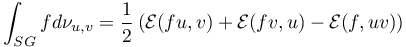
First of all, this looks superficially similar to the definition of the Christoffel Symbols in riemannian geometry. Points to anybody who figures out if there’s a real connection there.
Our Energy Measures
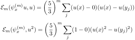
For our purposes, we consider energy measures of the form:
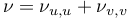
The integral of a function  with respect to
this energy measure will be:
with respect to
this energy measure will be:
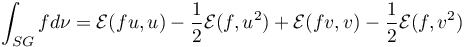
The level m approximation  to the energy
measure laplacian is:
to the energy
measure laplacian is:
It turns out that we can use what we know about the serpinski gasket to compute
the above expression exactly.
The function  is piecewise harmonic
on level m, being 1 at
is piecewise harmonic
on level m, being 1 at  and zero everywhere else.
Therefore, we can express the energy in a finite way:
and zero everywhere else.
Therefore, we can express the energy in a finite way:

We notice that almost every term in the sum of the energy is zero;
the only nonzero contributions come from the vertices
which are adjacent to .
If we let 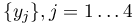 are the
neighboring vertices to
at level m:
are the
neighboring vertices to
at level m:
Which we can condense into a formula for the integral in question:
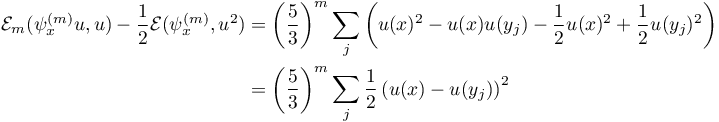
Therefore, the denominator of the energy measure now looks like this:
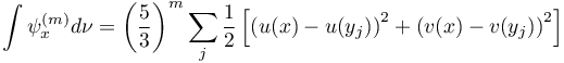
Using our new notation for the vertices, we can now write the energy laplacian with a nice pointwise formulation. Note that the normalization factors nicely cancel each other out.
With a formula like this, we can reasonable start to go around looking for a way to compute the laplaian matrix, and find out some of its properties including its eigenvalues and eigenvectors.
Computing the Energy Laplacian
Once we begin to start considering computing the energy laplacian matrix, we are presented with the problem of representing functions on the serpinski gasket.
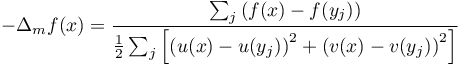
The graph representations at level 0 of the serpinski gasket is just a triangle:
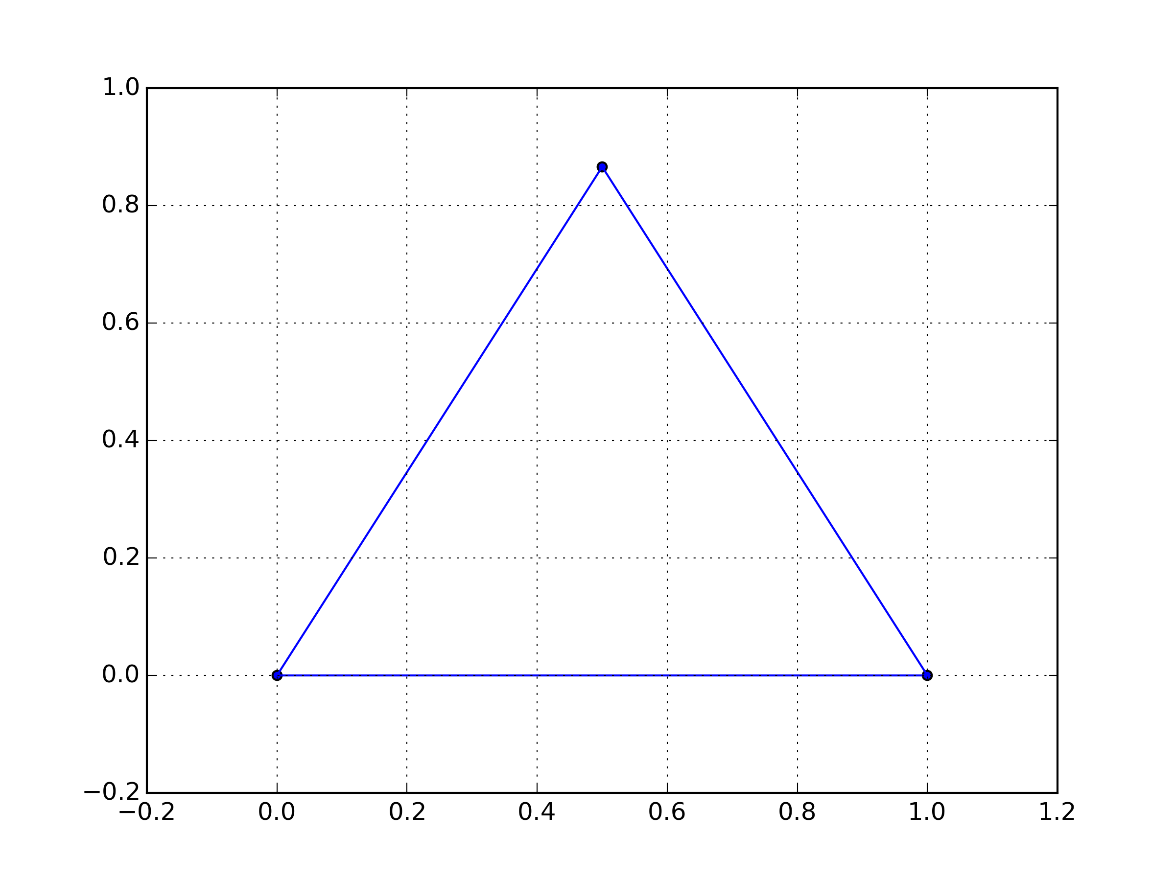
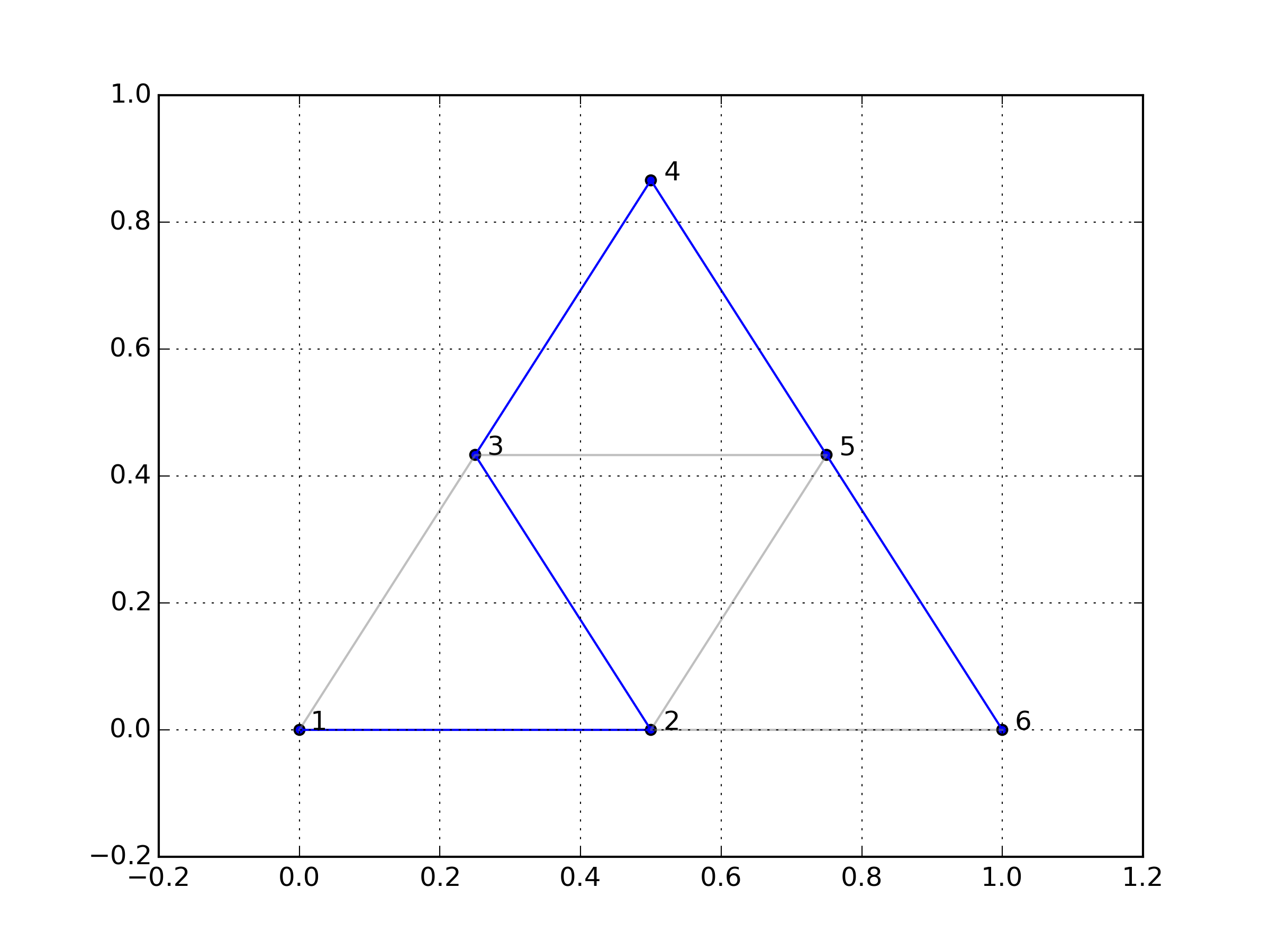
Add one more level:
And so on. If we’re working with an mth level approximation, we’re going to represent a function by storing an array of its values on the mth level graph approximation to the serpinski gasket. The formula we need to use includes differences between a vertex and its neighbors. Therefore, for every element of a function’s array representaiton, we need a way of efficiently figuring out which elements are adjacent to it.
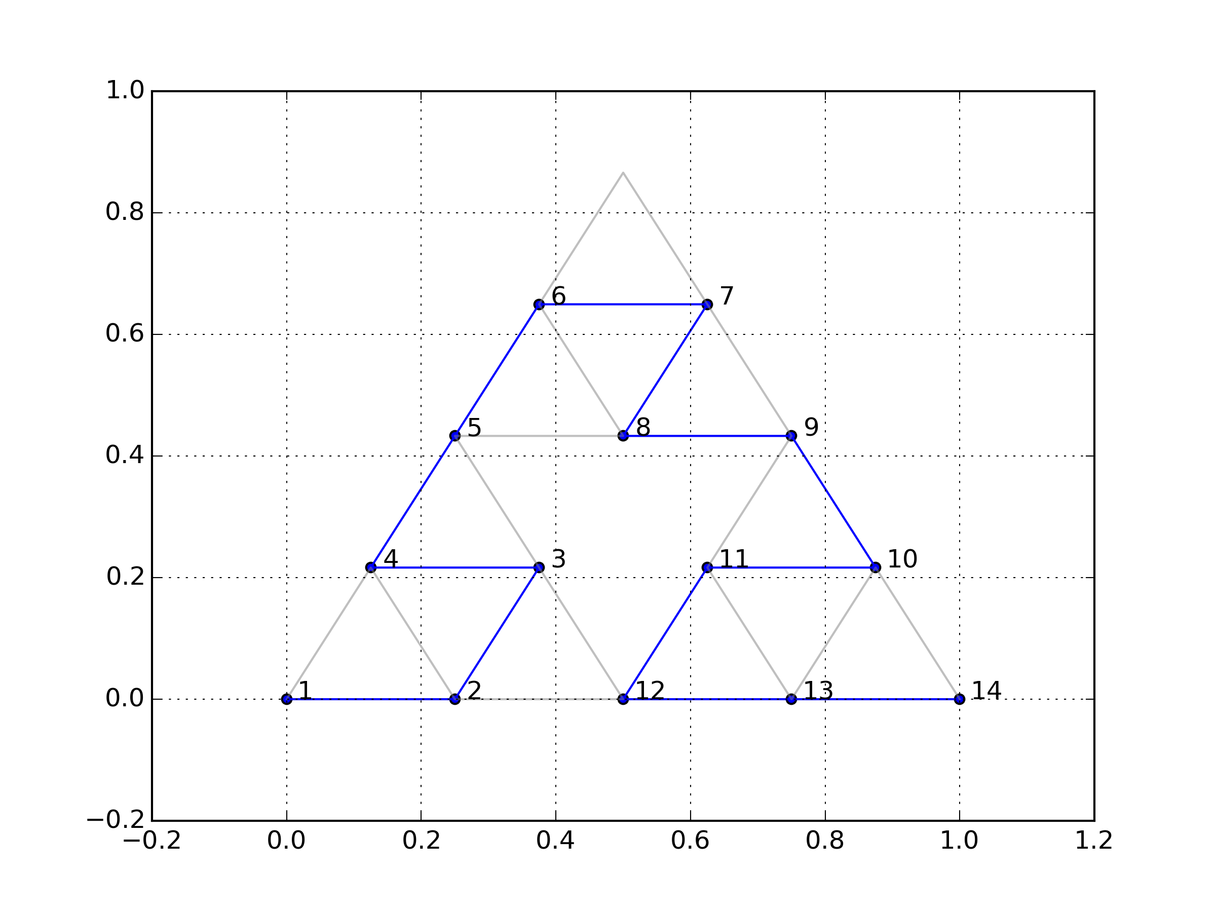
We accomplish this by indexing the serpinski gasket with a space-filling path. We will store an additional path in memory. We will use these two paths to find all adjacent vertices.
We will create a path which touches every point in the mth-level serpinski gasket exactly once (note that this path is a spanning tree). We will refer to this path as the “spiked path”. The path will start at one endpoint and finish at the other. We will then construct another path which starts and ends at the same points as the first path, does not touch the third boundary point at all, touches all of the vertices, and does not use any of the edges that the first path used. We will refer to this path as the “flat path”. We can inductively construct these paths. If we have constructed these paths according to plan, a point’s four neighbors will be its neighbors on the spiked path and flat path.
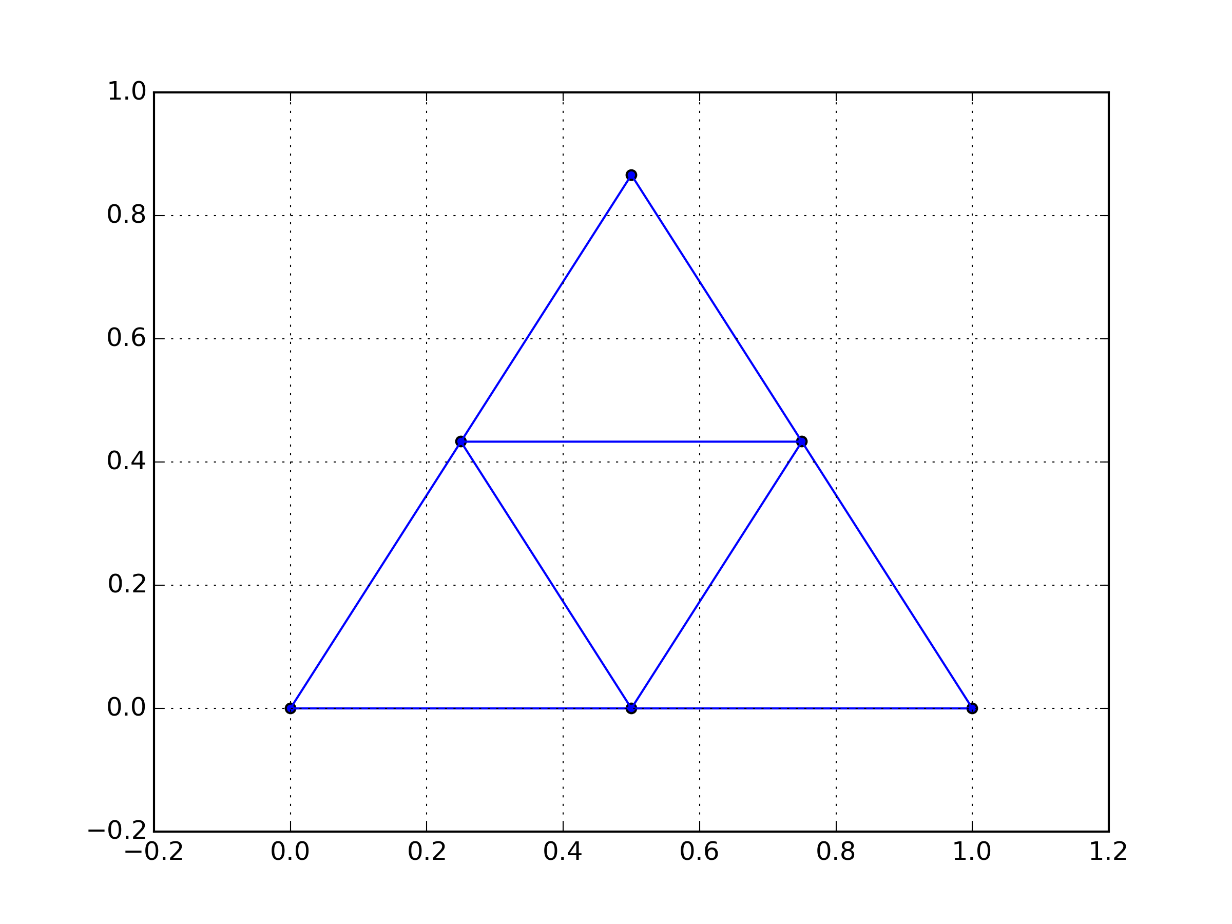
Base Case
Consider the paths:
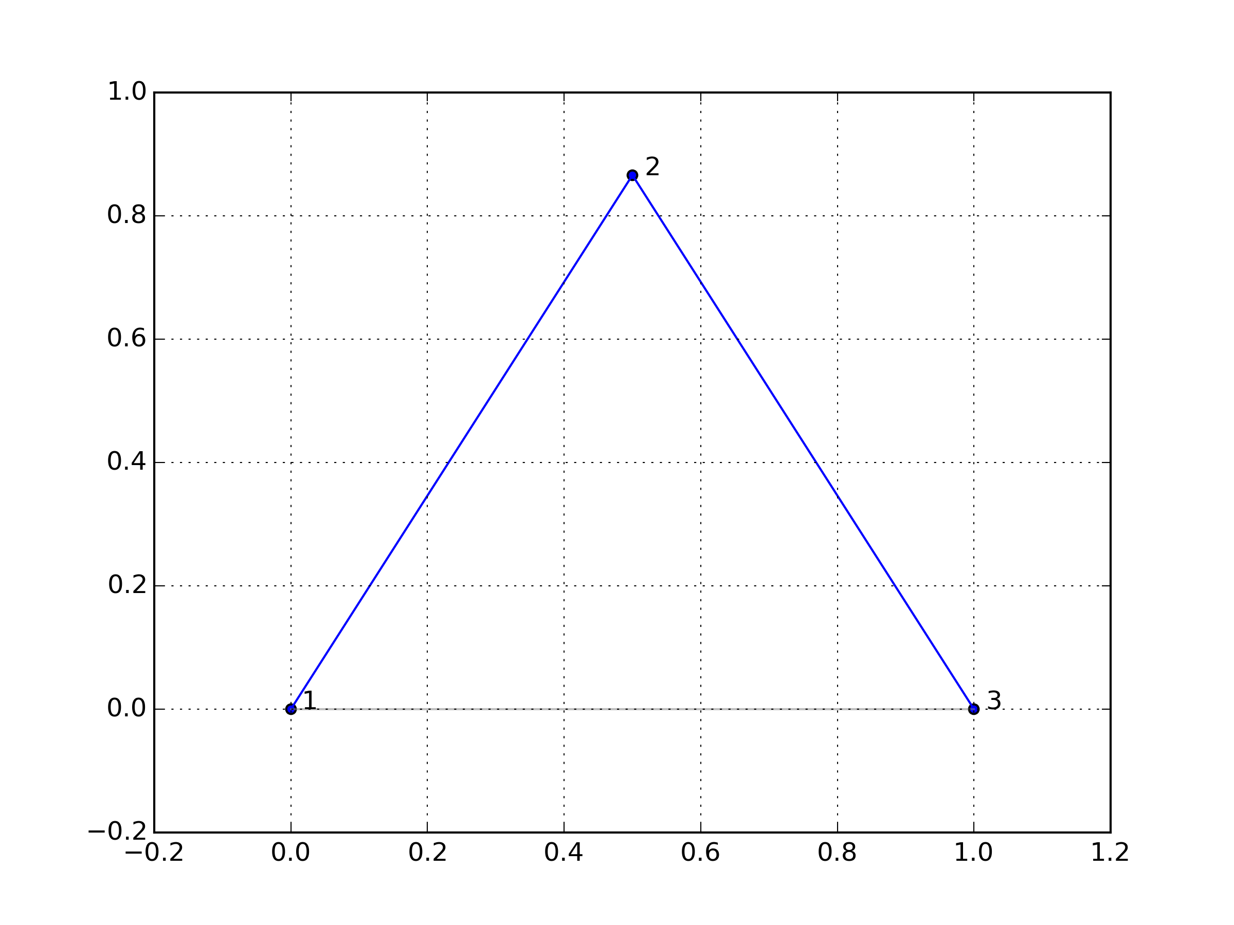
and
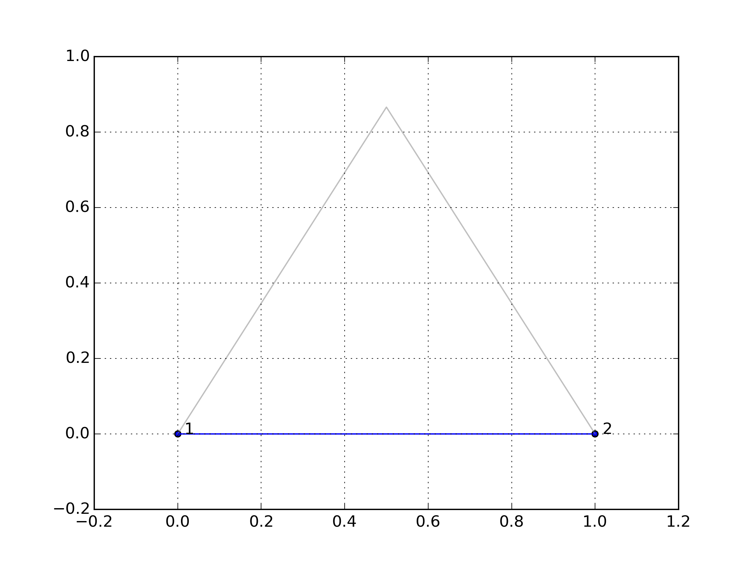
Note that the spiked path touches every point once. That path touches two corners once and one corner twice. Next, note that the flat path starts and ends at the same place as the spiked path, and doesn’t touch the one other vertex. It (trivially) touches every other point. Therefore, for the 0th level serpinski gasket, we have constructed paths which satisfy our conditions.
Inductive Step
We want to construct a pair of spiked path and flat path for the m+1-th level serpinski gasket, if the m-th level serpinski gasket has such a path. Note that if the m-th level serpinski gasket has a pair of spiked path and flat path, then we can put those paths into one of the three subtriangles of the serpinski gasket.
To construct a m+1-th spiked path, we join the lower left and upper vertices of the triangle with the m-th spiked path, so that the intersetion between the lower-left and lower-right triangles is covered by this path. Next, the upper triangle is traversed from left to right by a spiked path. Finally, the lower-left triangle is traversed from top to bottom-right by a flat path. This path joins the lower left with the lower right, and touches the top vertex, and is a spanning tree. Therefore, this path is an m+1-th spiked path.
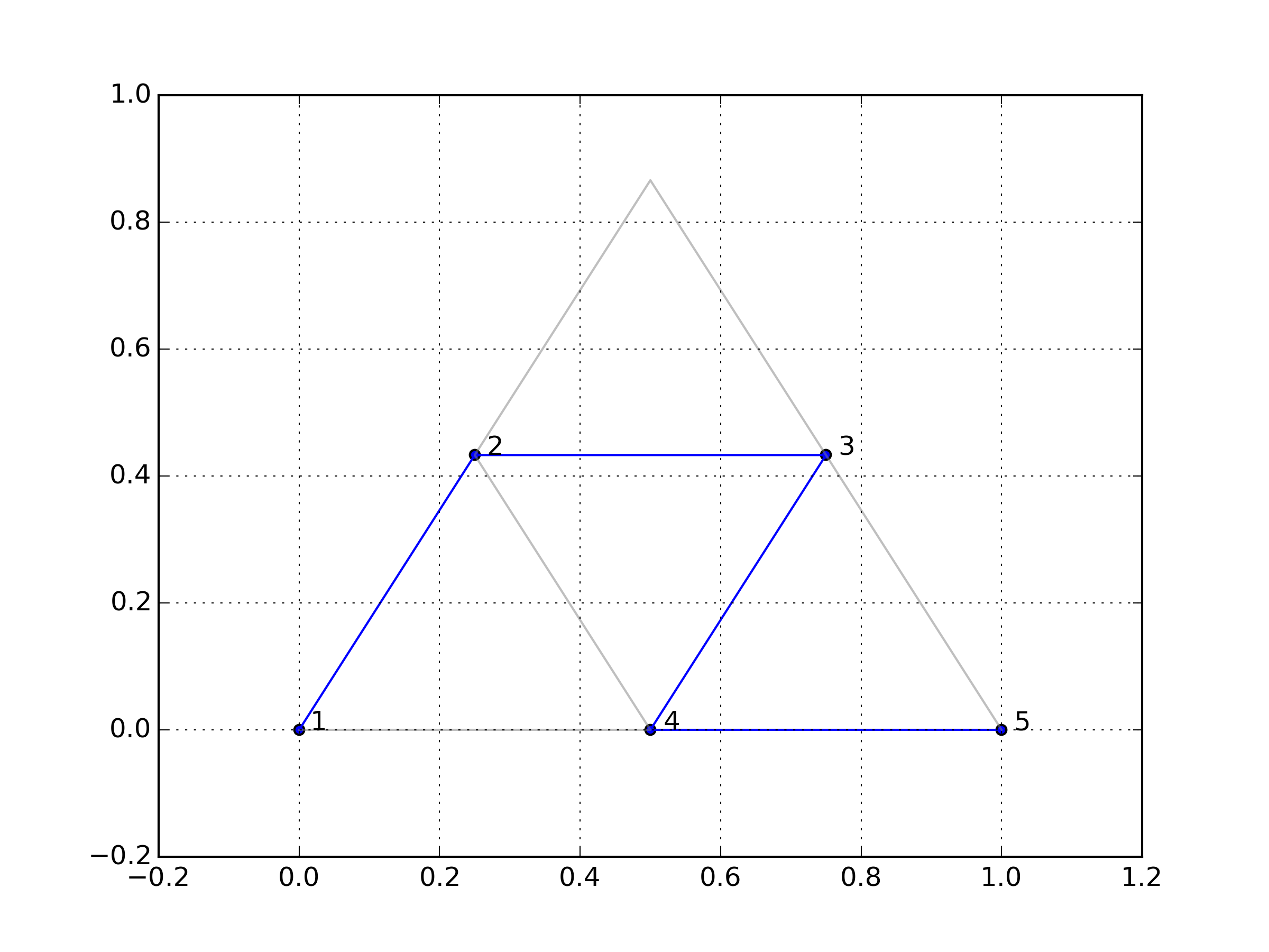
To construct an m+1-th flat path, we replace the spiked paths with flat paths in the previous construction. Note that since the m-th flat path is a flat path, when superimposed with the m-th spiked path they do not overlap, and together use all of the edges on the serpinski gasket. The m+1-th flat path does not include the top vertex because the m-th flat path doesn’t. This satisfies all of the properties that an m+1-th flat path needs to satisfy.
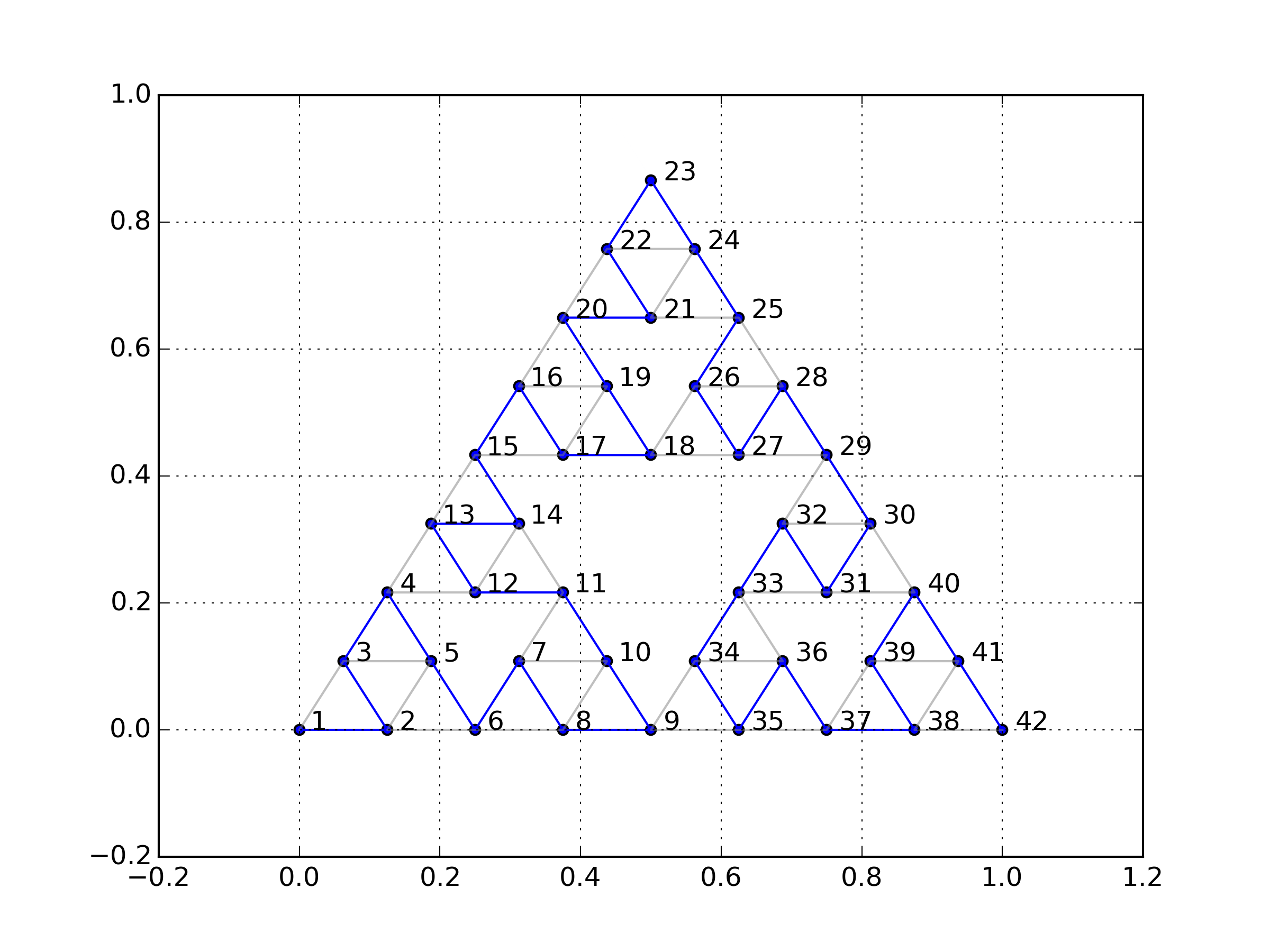
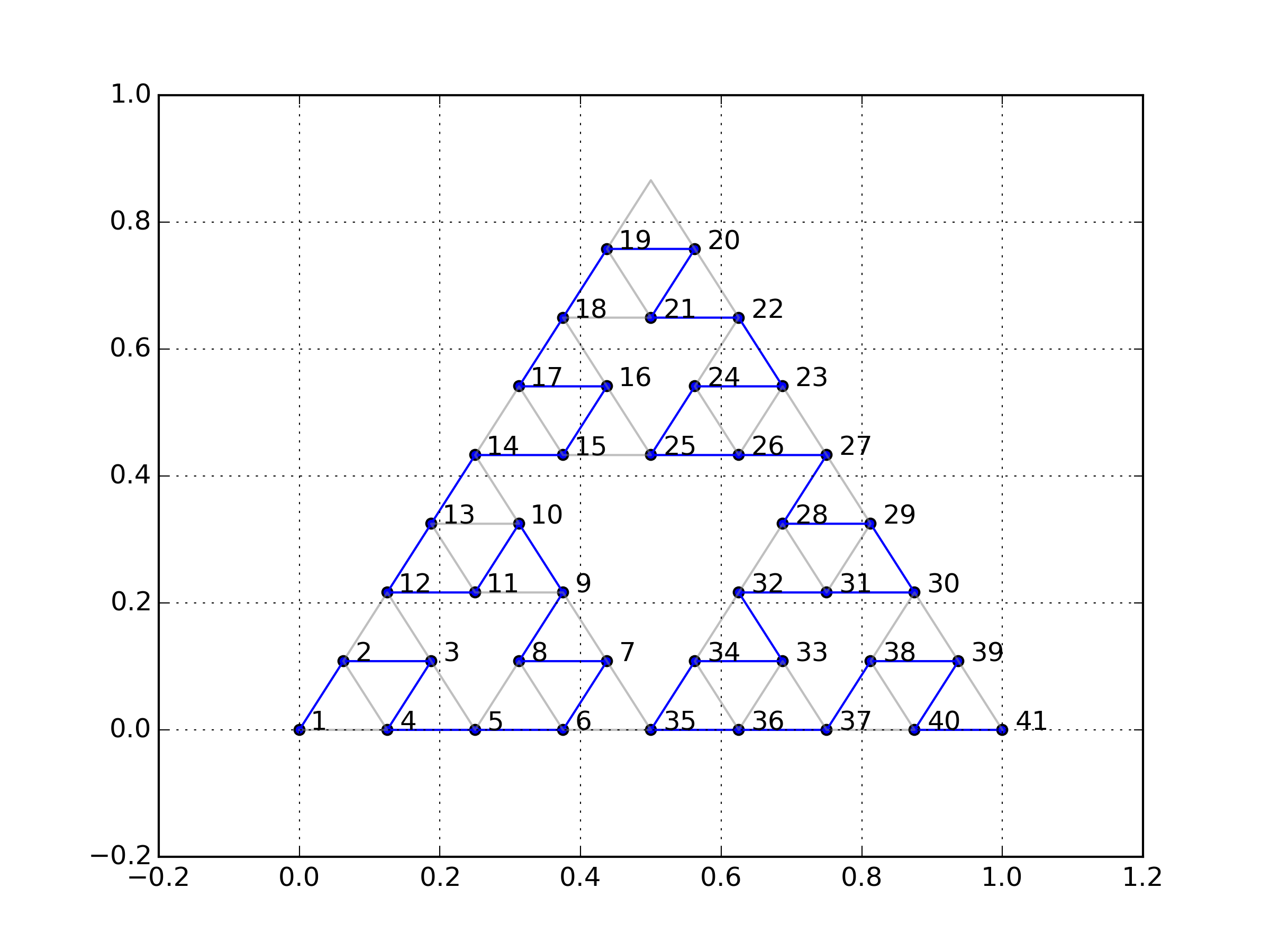
Below, we feature some of these paths.
1st spiked path
1st flat path
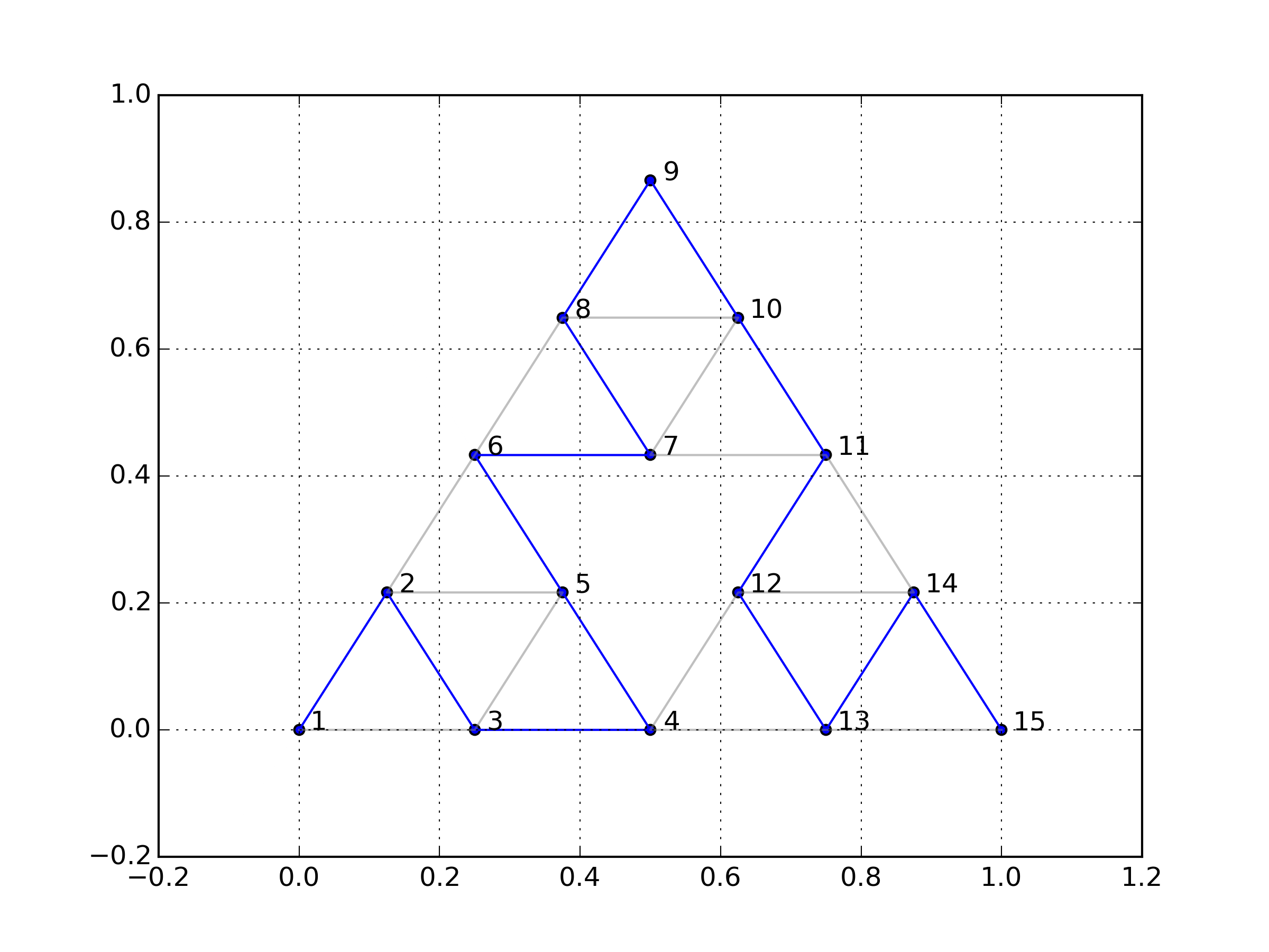
2nd spiked path
2nd flat path
3rd spiked path
3rd flat path
Using this layout scheme, we can extract some of the invariants which we care about. Let’s start with the eigenvalues:
When  ,
,
 , and
, and
